


Introduction
In our previous blog, we covered the basics of Pandas, focusing on operations like loading data, filtering, and grouping. Now, we’ll dive into advanced functionalities that Pandas offers, which are crucial for more complex data manipulation and analysis.
In this blog, we’ll cover:
- Handling missing data
- Merging and concatenating DataFrames
- Working with pivot tables
- Applying custom functions using
apply() - Time series analysis
- Using window functions for rolling calculations
To demonstrate these operations, we’ll use a sample employee dataset stored in a CSV file.
1. Loading a CSV File into Pandas
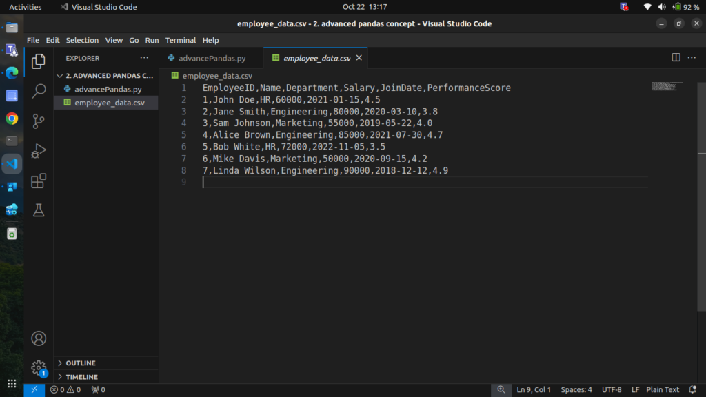
We’ll use the following employee data stored in a CSV file, Save this data as employee_data.csv.
EmployeeID,Name,Department,Salary,JoinDate,PerformanceScore
1,John Doe,HR,60000,2021-01-15,4.5
2,Jane Smith,Engineering,80000,2020-03-10,3.8
3,Sam Johnson,Marketing,55000,2019-05-22,4.0
4,Alice Brown,Engineering,85000,2021-07-30,4.7
5,Bob White,HR,72000,2022-11-05,3.5
6,Mike Davis,Marketing,50000,2020-09-15,4.2
7,Linda Wilson,Engineering,90000,2018-12-12,4.9
Step 1: Loading the CSV Data
import pandas as pd

# Load the CSV file into a DataFrame
df = pd.read_csv('employee_data.csv')

# Display the DataFrame
print(df)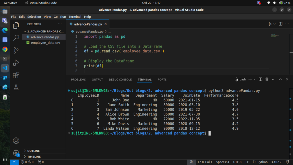
Now that we have our data loaded, let’s explore more advanced operations.
2. Handling Missing Data
In real-world datasets, it’s common to encounter missing data. Pandas provides several methods to handle these missing values. Let’s introduce some missing data into our dataset and demonstrate how to deal with it. we are gonna use of numpy to add missing values in columns
Step 2.1: Introducing Missing Data
import numpy as np

# Introduce missing values in the 'Salary' and 'PerformanceScore' columns
df.loc[2, 'Salary'] = np.nan
df.loc[5, 'PerformanceScore'] = np.nan

# Display the DataFrame with missing values
print(df)
Output
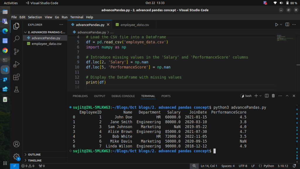
Now we have missing values in the Salary and PerformanceScore columns.
Step 2.2: Handling Missing Values
We can handle missing data in various ways:
- Filling missing values with a specific value or the median of the column
- Forward filling values
- Dropping rows with missing values
2.2.1 Filling Missing Values with the Median
# Fill missing 'Salary' with the median value of the column
df['Salary'] = df['Salary'].fillna(df['Salary'].median())

# Display the updated DataFrame
print(df)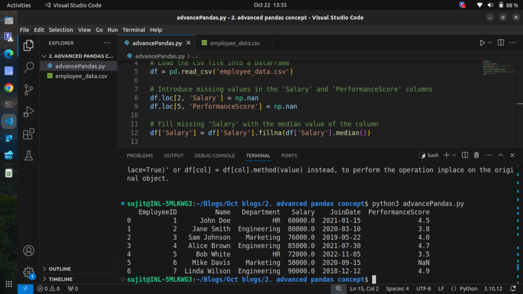
2.2.2 Forward Filling Missing Values
import pandas as pd
import numpy as np

# Load the CSV file into a DataFrame
df = pd.read_csv('employee_data.csv')

# Introduce missing values in the 'Salary' and 'PerformanceScore' columns
df.loc[2, 'Salary'] = np.nan
df.loc[5, 'PerformanceScore'] = np.nan

# Fill missing 'Salary' with the median value of the column
df['Salary'] = df['Salary'].fillna(df['Salary'].median())

# Fill missing values in 'PerformanceScore' with the median
df['PerformanceScore'] = df['PerformanceScore'].fillna(df['PerformanceScore'].median())

# Display the updated DataFrame
print(df)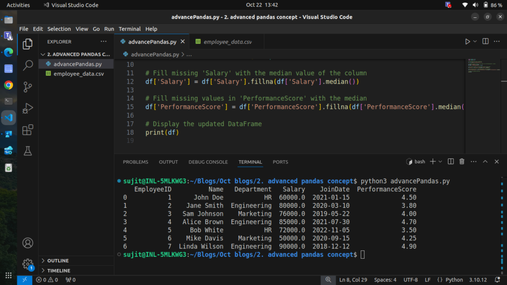
Now the missing data has been handled effectively.
3. Merging and Concatenating DataFrames
Merging DataFrames is essential when you need to combine data from different sources. We can use the merge() function for this purpose.
Step 3.1: Merging DataFrames
Let’s say we have another DataFrame containing bonus data for each employee:
# Create a DataFrame with bonus data
bonus_data = pd.DataFrame({
    'EmployeeID': [1, 2, 3, 4, 5, 6, 7],
    'Bonus': [5000, 8000, 3000, 10000, 2000, 2500, 15000]
})

# Merge with the employee DataFrame
merged_df = pd.merge(df, bonus_data, on='EmployeeID', how='left')

# Display the merged DataFrame
print(merged_df)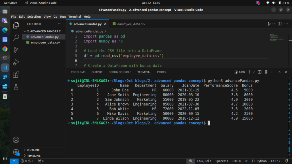
We have successfully added the bonus data for each employee.
4. Pivot Tables
Pivot tables are powerful tools for summarizing data. Let’s create a pivot table to summarize the average salary by department.
Step 4.1: Creating a Pivot Table
# Create a pivot table to summarize average salary by department
pivot_table = df.pivot_table(values='Salary', index='Department', aggfunc='mean')

# Display the pivot table
print(pivot_table)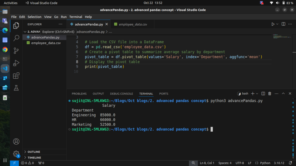
This pivot table shows the average salary for each department.
5. Applying Custom Functions with apply()
We can use the apply() function to execute custom operations on DataFrame columns or rows.
Step 5.1: Applying a Custom Function
Let’s create a custom function to categorize performance scores.
# Define a custom function to categorize performance
def categorize_performance(score):
    if score < 3.5:
        return 'Needs Improvement'
    elif score < 4.5:
        return 'Meets Expectations'
    else:
        return 'Exceeds Expectations'

# Apply the custom function to the 'PerformanceScore' column
df['Performance_Category'] = df['PerformanceScore'].apply(categorize_performance)

# Display the updated DataFrame
print(df)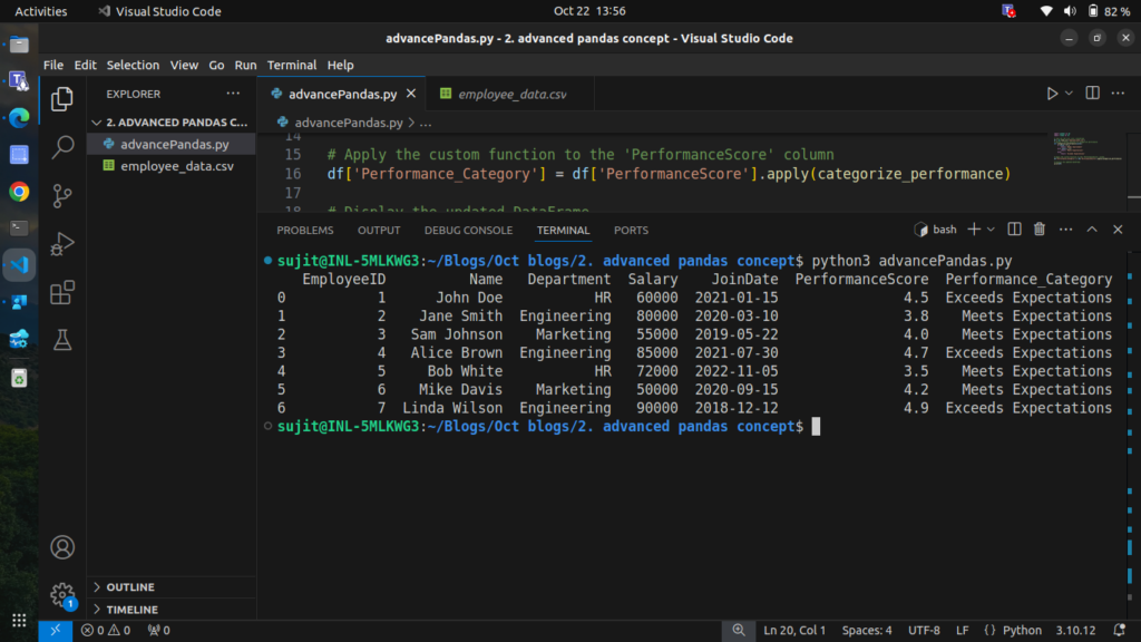
The performance of each employee has been categorized successfully.
6. Time Series Analysis
Pandas makes working with time-series data straightforward. Let’s analyze employee joining dates.
At this point, the JoinDate column is treated as a string, so you can’t easily perform operations like sorting, filtering by date range, or extracting year/month values.
Step 6.1: Converting Strings to Datetime Format
# Convert 'JoinDate' column to datetime format
df['JoinDate'] = pd.to_datetime(df['JoinDate'])

# Display the updated DataFrame
print(df)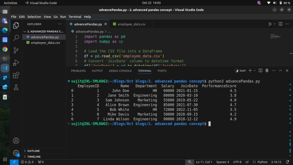
After converting the JoinDate column to a datetime format, we can perform various time-related analyses.
Step 6.2: Analyzing Time Series Data
We can extract information from the JoinDate, such as the year or month of joining.
# Extract the year and month from the 'JoinDate'
df['JoinYear'] = df['JoinDate'].dt.year
df['JoinMonth'] = df['JoinDate'].dt.month

# Display the updated DataFrame
print(df)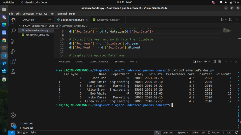
7. Rolling Window Calculations
Rolling window functions are useful for calculating statistics over a moving window of data. Let’s calculate the rolling average salary for employees based on their joining date.
Step 7.1: Calculating Rolling Average Salary
# Sort the DataFrame by 'JoinDate'
df.sort_values('JoinDate', inplace=True)

# Calculate the rolling average salary over a 3-employee window
df['Rolling_Avg_Salary'] = df['Salary'].rolling(window=3).mean()

# Display the DataFrame with the rolling average
print(df)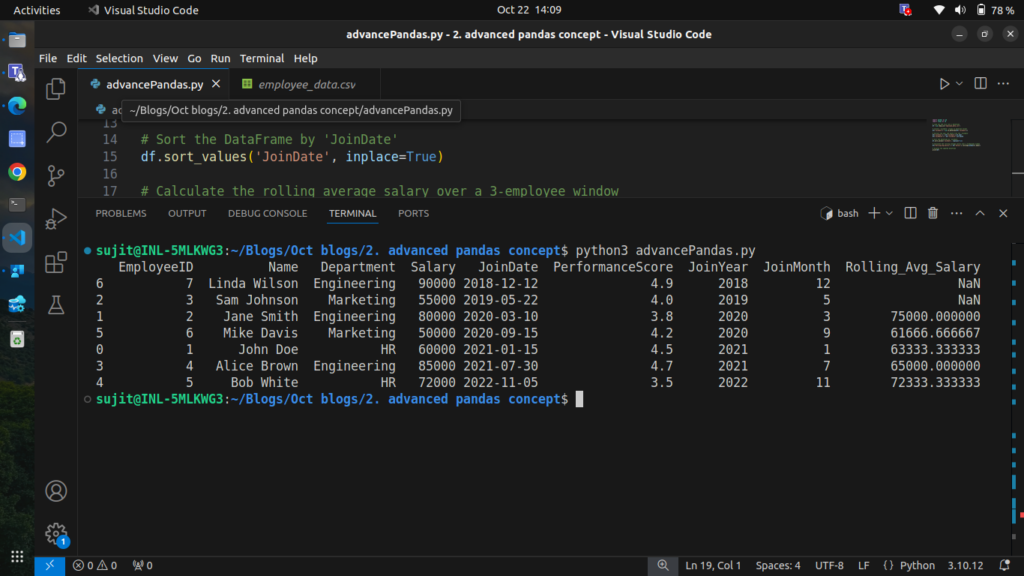
here is the complete code for this blog:
import pandas as pd
import numpy as np

# Step 1: Load the CSV file into a DataFrame
df = pd.read_csv('employee_data.csv')

# Display the original DataFrame
print("Original DataFrame:")
print(df)

# Step 2: Introduce missing values in 'Salary' and 'PerformanceScore'
df.loc[2, 'Salary'] = np.nan
df.loc[5, 'PerformanceScore'] = np.nan

# Display the DataFrame with missing values
print("\nDataFrame with Missing Values:")
print(df)

# Step 2.2: Handling Missing Values
# Fill missing 'Salary' with the median value of the column
df['Salary'].fillna(df['Salary'].median(), inplace=True)

# Forward fill missing 'PerformanceScore' values
df['PerformanceScore'].fillna(method='ffill', inplace=True)

# Display the updated DataFrame
print("\nDataFrame after Handling Missing Values:")
print(df)

# Step 3: Create a DataFrame with bonus data
bonus_data = pd.DataFrame({
    'EmployeeID': [1, 2, 3, 4, 5, 6, 7],
    'Bonus': [5000, 8000, 3000, 10000, 2000, 2500, 15000]
})

# Merge with the employee DataFrame
merged_df = pd.merge(df, bonus_data, on='EmployeeID', how='left')

# Display the merged DataFrame
print("\nMerged DataFrame with Bonus Data:")
print(merged_df)

# Step 4: Create a pivot table to summarize average salary by department
pivot_table = df.pivot_table(values='Salary', index='Department', aggfunc='mean')

# Display the pivot table
print("\nPivot Table of Average Salary by Department:")
print(pivot_table)

# Step 5: Define a custom function to categorize performance
def categorize_performance(score):
    if score < 3.5:
        return 'Needs Improvement'
    elif score < 4.5:
        return 'Meets Expectations'
    else:
        return 'Exceeds Expectations'

# Apply the custom function to the 'PerformanceScore' column
df['Performance_Category'] = df['PerformanceScore'].apply(categorize_performance)

# Display the updated DataFrame with performance categories
print("\nDataFrame with Performance Categories:")
print(df)

# Step 6: Convert 'JoinDate' column to datetime format
df['JoinDate'] = pd.to_datetime(df['JoinDate'])

# Extract the year and month from the 'JoinDate'
df['JoinYear'] = df['JoinDate'].dt.year
df['JoinMonth'] = df['JoinDate'].dt.month

# Display the updated DataFrame
print("\nDataFrame with Join Year and Month:")
print(df)

# Step 7: Sort the DataFrame by 'JoinDate'
df.sort_values('JoinDate', inplace=True)

# Calculate the rolling average salary over a 3-employee window
df['Rolling_Avg_Salary'] = df['Salary'].rolling(window=3).mean()

# Display the DataFrame with the rolling average
print("\nDataFrame with Rolling Average Salary:")
print(df)
Conclusion
In this blog, we explored advanced Pandas operations that can significantly enhance your data analysis capabilities. We covered:
- Handling missing data effectively
- Merging and concatenating DataFrames
- Creating insightful pivot tables
- Applying custom functions with
apply() - Performing time series analysis
- Utilizing rolling window calculations
These techniques are essential for anyone looking to perform in-depth data analysis in Python using Pandas.