Data Lakehouse on AWS: Leverage Glue Notebooks for Data Workflow Automation (Part 2)

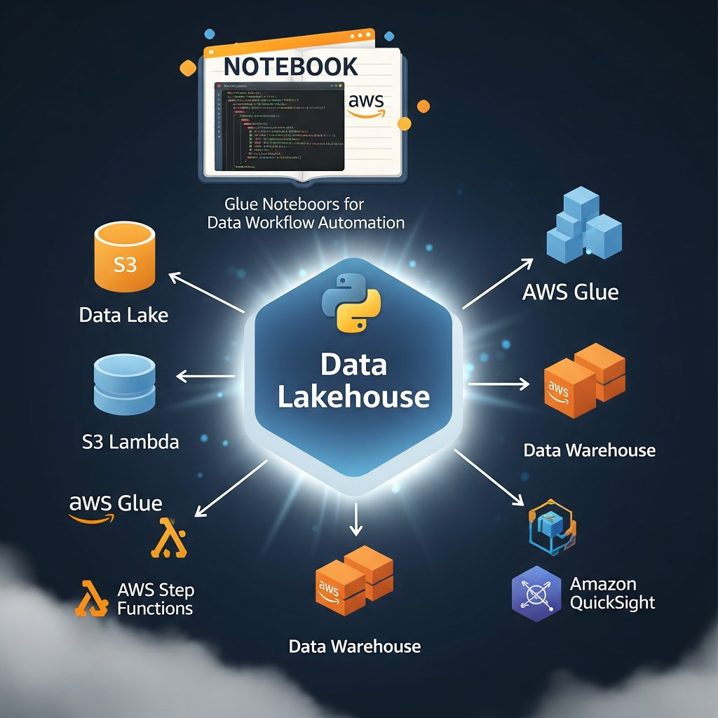
Continuing from part 1, this section will focus on establishing a medallion architecture ETL pipeline: Raw -> Bronze -> Silver -> Gold using Glue notebooks. Additionally, we will create a Glue workflow that outlines the complete process for the initial data workflow. To explore insights from the data model in the gold layer, we will utilize Athena to conduct several ad-hoc queries. Furthermore, to comprehend why Apache Iceberg is favored in contemporary Lakehouse architectures, we will examine the metadata it generates in S3 buckets.

Understand data model and raw data structure in this article

To fully understand the logic that will be implemented in the notebooks below, we need to understand the structure of the raw JSON data, as well as the target data model that the entire workflow is aiming for.

Explain the JSON structure from the source

Here is an example of the raw JSON file as the resource to feed the data pipeline:

[
    {
        "category": [
            {
                "category_id": "11035567",
                "category_name": "Thời Trang Nam",
                "parent_id": -1
            },
            {
                "category_id": "11035572",
                "category_name": "Áo Vest và Blazer",
                "parent_id": "11035567"
            }
        ],
        "url": "https://shopee.vn/B%E1%BB%99-Vest-Nam-Cao-C%E1%BA%A5p-M%C3%A0u-Tr%E1%BA%AFng-B%E1%BB%99-suit-nam-H%C3%A0n-Qu%E1%BB%91c-m%C3%A0u-tr%E1%BA%AFng-(-V%E1%BA%A3i-X%E1%BB%8Bn-2-L%E1%BB%9Bp-)-i.568109992.29951402391?sp_atk=229a485e-86c7-4bcd-afb5-8e69d368acd9&xptdk=229a485e-86c7-4bcd-afb5-8e69d368acd9",
        "image": "https://down-vn.img.susercontent.com/file/sg-11134201-7rd4n-lvxh4rvz0mpo36_tn",
        "title": "Bộ Vest Nam Cao Cấp Màu Trắng, Bộ suit nam Hàn Quốc màu trắng ( Vải Xịn 2 Lớp )",
        "promotions": [
            "Giảm ₫5k"
        ],
        "price": {
            "current_price": "609.000",
            "original_price": "₫870.000",
            "discount_rate": "-30%"
        },
        "sold": "",
        "location": "Hưng Yên"
    },
    {
        "category": [
            {
                "category_id": "11035567",
                "category_name": "Thời Trang Nam",
                "parent_id": -1
            },
            {
                "category_id": "11035572",
                "category_name": "Áo Vest và Blazer",
                "parent_id": "11035567"
            }
        ],
        "url": "https://shopee.vn/B%E1%BB%99-%C4%91%E1%BB%93-Slim-Fit-B%E1%BB%99-%C4%91%E1%BB%93-m%C3%A0u-tr%C6%A1n-B%E1%BB%99-%C4%91%E1%BB%93-2-m%C3%B3n-s%C3%A0nh-%C4%91i%E1%BB%87u-B%E1%BB%99-%C4%91%E1%BB%93-nam-Slim-Fit-Ve-%C3%A1o-kho%C3%A1c-gi%E1%BB%AFa-cao-Qu%E1%BA%A7n-m%C3%A0u-tr%C6%A1n-b%E1%BA%A3o-h%E1%BB%99-lao-%C4%91%E1%BB%99ng-i.130953959.29901695241?sp_atk=565680b3-eaac-4ebc-9631-274373ffc143&xptdk=565680b3-eaac-4ebc-9631-274373ffc143",
        "image": "https://down-vn.img.susercontent.com/file/sg-11134201-7rd6d-lw3brv77afmmac_tn",
        "title": "Bộ đồ Slim Fit Bộ đồ màu trơn Bộ đồ 2 món sành điệu Bộ đồ nam Slim Fit Ve áo khoác giữa cao Quần màu trơn bảo hộ lao động",
        "promotions": [
            "Giảm ₫27k"
        ],
        "price": {
            "current_price": "327.145",
            "original_price": "₫467.350",
            "discount_rate": "-30%"
        },
        "sold": "",
        "location": "Nước ngoài"
    }
]

These source files are taken from an e-commerce site. Their JSON structure is quite clean; it is simply a string of many objects, each representing product information:

From the original data, it will be cleaned and processed through a designated pipeline. The cleaned data will then populate a data model to facilitate data analysis.

Overview of the final data model

The Data model is located at the gold layer and is designed according to the Kimball methodology. Let’s have a look at it:

Configuration updates from Part 1

We did some core services configuration in Part 1. To align with the new part, we will add some modifications to the existing setting.

{
	"Version": "2012-10-17",
	"Statement": [
		{
			"Sid": "AllowPassSelfToGlue",
			"Effect": "Allow",
			"Action": "iam:PassRole",
			"Resource": "arn:aws:iam::058432329112:role/EcomLakehouseGlueRole",
			"Condition": {
				"StringEquals": {
					"iam:PassedToService": "glue.amazonaws.com"
				}
			}
		}
	]
}

Create notebooks as jobs & implement logics for all layers

Finally, it’s time to dive into the practical aspects. To ensure our jobs run as efficiently as possible, we’ll leverage Glue Notebooks, which allow for executing code blocks individually. This capability is invaluable for data exploration, process development, and iterative refinement.

1. Create `raw_to_bronze` notebooks

1.1. Create a notebook in AWS Glue Studio

• Navigate to AWS Glue –> Select ETL jobs.
• On Create job section –> Choose Notebook –> A pop-up will show up.
• Next, select Start fresh option –> choose EcomLakehouseGlueRole IAM role.
• Click on Create Notebook –> Rename the title to raw_to_bronze
• Wait for a few minutes for the notebook to start.

The default capacity of a notebook is 5 workers. We can change the notebook configurations by adjusting the arguments of %magic commands inside each one.

TIPs: Notebooks are charged based on how long they run (per minute). So click Stop Notebook when not in use to save costs.

1.2. Implement the raw to bronze logic, cell by cell

# initial configuration
%%configure
{
  "--datalake-formats": "iceberg",
  "--conf": "spark.sql.extensions=org.apache.iceberg.spark.extensions.IcebergSparkSessionExtensions --conf spark.sql.catalog.glue_catalog=org.apache.iceberg.spark.SparkCatalog --conf spark.sql.catalog.glue_catalog.warehouse=s3://ecom-analyzer-lakehouse/ --conf spark.sql.catalog.glue_catalog.catalog-impl=org.apache.iceberg.aws.glue.GlueCatalog --conf spark.sql.catalog.glue_catalog.io-impl=org.apache.iceberg.aws.s3.S3FileIO"
} # the important config to make the following code use modern iceberg APIs

%idle_timeout 2880 # time out value, in minutes
%glue_version 5.0 # glue version, use the latest
%worker_type G.1X # worker type, could increase
%number_of_workers 5 # number of spark workers, could increase

# Initialize Spark with optimizations for 2GB+ JSON processing
import sys
from awsglue.transforms import *
from awsglue.utils import getResolvedOptions
from pyspark.context import SparkContext
from awsglue.context import GlueContext
from awsglue.job import Job
from pyspark.sql import SparkSession
from pyspark.sql.functions import (
    current_timestamp, lit, col, input_file_name, to_date,
    explode, regexp_extract, split, trim, concat_ws, concat, size, expr,
    coalesce, when
)
from datetime import datetime

# Initialize Glue Context
sc = SparkContext.getOrCreate()
glueContext = GlueContext(sc)
spark = glueContext.spark_session
job = Job(glueContext)

print("🚀 Initializing optimized Spark session for bronze layer...")

# Global variables init
BUCKET_NAME = "ecom-analyzer-lakehouse"
RAW_PATH = f"s3://{BUCKET_NAME}/raw/"

# Bronze Layer Database Configuration
BRONZE_DATABASE = "ecom_bronze"
BRONZE_LOCATION = f"s3://{BUCKET_NAME}/bronze/"

BRONZE_TABLES = {
    "raw_data": {
        "partitions": ["ingestion_date"]
    },
    "products": {
        "partitions": ["ingestion_date"]
    },
    "categories": {
        "partitions": ["ingestion_date"]
    }
}

# Get job parameters
try:
    args = getResolvedOptions(sys.argv, ['JOB_NAME', 'raw_path', 'bucket_name'])
    RAW_PATH = args.get('raw_path', RAW_PATH)
    BUCKET_NAME = args.get('bucket_name', BUCKET_NAME)
    job.init(args['JOB_NAME'], args)
    
    # Update all paths if bucket changed
    if BUCKET_NAME != "ecom-analyzer-lakehouse":
        BRONZE_LOCATION = f"s3://{BUCKET_NAME}/bronze/"
        for table_name in BRONZE_TABLES:
            BRONZE_TABLES[table_name]["location"] = f"{BRONZE_LOCATION}{table_name}/"
except:
    print("Running in notebook mode")

print(f"🗂️  Bronze Database: {BRONZE_DATABASE}")
print(f"📍 Database Location: {BRONZE_LOCATION}")
print(f"📁 Raw Data Source: {RAW_PATH}")
print(f"📊 Tables: {len(BRONZE_TABLES)} bronze tables configured")

# Create a new database for bronze layer using spark SQL
print(f"🗄️  Creating bronze database: {BRONZE_DATABASE}")
spark.sql(f"CREATE DATABASE IF NOT EXISTS {BRONZE_DATABASE} LOCATION '{BRONZE_LOCATION}'")
spark.sql(f"USE {BRONZE_DATABASE}")
print(f"✅ Bronze database ready at: {BRONZE_LOCATION}")

# The first way of saving files (Use native Spark API)
def create_iceberg_table_v1(df, table_name, config):
    """Create table with Iceberg format using legacy API"""
    partitions = config["partitions"]
    
    print(f"\n📋 Creating table: {table_name}")
    
    try:
        # Write data first
        writer = df.write.format("iceberg").mode("overwrite")
        if partitions:
            writer = writer.partitionBy(*partitions)
        
        # Use full catalog path
        full_table_name = f"glue_catalog.{BRONZE_DATABASE}.{table_name}"
        writer.saveAsTable(full_table_name)
        print(f"✅ Iceberg table created successfully!")
        return True
    except Exception as e:
        print(f"❌ Error: {str(e)}")
        return False

# The second way of creating a table in Iceberg format (Use iceberg API)
def create_iceberg_table_v2(df, table_name, config):
    """Create table with Iceberg format using morden API"""
    partitions = config["partitions"]

    print(f"\n📋 Creating table: {table_name}")

    try:
        # Use full catalog path
        full_table_name = f"glue_catalog.{BRONZE_DATABASE}.{table_name}"
        
        # Drop table if exists
        spark.sql(f"DROP TABLE IF EXISTS {full_table_name}")
        
        # Write data first
        writer = df.writeTo(full_table_name).using("iceberg")
        
        table_properties = {
            # Format version 2 - support row-level operations (UPDATE, DELETE, MERGE)
            "format-version": "2",

            # File size optimization (128MB optimal cho S3 + Athena)
            "write.target-file-size-bytes": "134217728",  # 128MB

            # Metadata cleanup - for cost optimization
            "write.metadata.delete-after-commit.enabled": "true",
            "write.metadata.previous-versions-max": "15"
        }

        # Apply table properties
        for key, value in table_properties.items():
            writer = writer.tableProperty(key, value)
        
        if partitions:
            writer = writer.partitionedBy(*partitions)

        writer.create()
        print(f"✅ Iceberg table created successfully!")
        return True

    except Exception as e:
        print(f"❌ Error: {str(e)}")
        return False

# Read raw JSON files from raw layer
print("Reading raw JSON files...")
raw_df = spark.read \
    .option("multiline", "true") \
    .json(f"{RAW_PATH}/products-2024-06-26*.json")

# Add metadata columns
raw_df = raw_df \
    .withColumn("ingestion_timestamp", current_timestamp()) \
    .withColumn("source_file", input_file_name()) \
    .withColumn("ingestion_date", to_date(current_timestamp())) \
    .withColumn("job_run_id", lit('raw_to_bronze_' + datetime.now().strftime("%Y%m%d_%H%M%S")))

print(f"Total records read: {raw_df.count()}")
raw_df.printSchema() # for profiling or schema checking

# transform the JSON format to an iceberg table
# then we can use Athena for fast and convenient queries
print("\n=== Raw Data Table ===")
create_iceberg_table_v1(raw_df, "raw_data", BRONZE_TABLES["raw_data"])

# Extract the products related only to the separated table
# Make it easier to clean data in the silver layer
products_df = raw_df.select(
    # Extract shop_id and product_code from URL using improved regex
    regexp_extract(col("url"), r'i\.(\d+)\.(\d+)', 1).alias("shop_id"),
    regexp_extract(col("url"), r'i\.(\d+)\.(\d+)', 2).alias("product_code"),

    # Product information
    col("url").alias("product_url"),
    col("image").alias("product_image"),
    col("title").alias("product_name"),
    col("promotions"),

    # Price information (keep as strings for bronze layer)
    col("price.current_price").alias("current_price"),
    col("price.original_price").alias("original_price"),
    col("price.discount_rate").alias("discount_rate"),

    # Sales and location
    col("sold"),
    col("location"),

    # Category information (preserve nested structure)
    col("category"),

    # Metadata
    col("ingestion_timestamp"),
    col("source_file"),
    col("ingestion_date"),
    col("job_run_id")
).filter(
    # Filter out records without valid product codes
    col("product_code").isNotNull() & 
    (col("product_code") != "") &
    col("product_name").isNotNull()
)

products_df.printSchema()

print("\n=== Products Table using v2 ===")
create_iceberg_table_v2(products_df, "products", BRONZE_TABLES["products"])

# Create an isolated table for all product categories also
categories_df = raw_df.select(
    explode(col("category")).alias("category_data"),
    col("ingestion_timestamp"),
    col("ingestion_date"),
    col("job_run_id")
).select(
    col("category_data.category_id").alias("category_code"),
    col("category_data.category_name"),
    col("category_data.parent_id").alias("parent_code"),
    col("ingestion_timestamp"),
    col("ingestion_date"),
    col("job_run_id")
).filter(
    # Filter out invalid categories
    col("category_code").isNotNull() &
    col("category_name").isNotNull()
).dropDuplicates(["category_code"])
categories_df.printSchema()

print("\n=== Categories Table v2===")
create_iceberg_table_v2(categories_df, "categories", BRONZE_TABLES["categories"])

You could find the complete notebook flie here: raw_to_bronze.ipynb

2. Create `bronze_to_silver` notebooks in the silver database

The processing logic of bronze_to_silver has much in common with raw_to_bronze at the beginning. However, the difference comes from the data cleaning part, where you need to create a few user-defined functions to handle the junk data.

# Define UDFs for data transformation
def extract_sold_number(s: str) -> int:
    """Extract sold number from string, handling 'k' notation"""
    if not s:
        return 0
    s = str(s).strip()
    if not s:
        return 0
    
    # Extract numeric part
    match = re.search(r'(\d+[.,]?\d*)[kK]?', s)
    if not match:
        return 0
    
    num_str = match.group(1)
    # Handle 'k' notation
    if 'k' in s.lower():
        if '.' in num_str or ',' in num_str:
            # For values like "1.5k" or "1,5k"
            num_str = num_str.replace('.', '').replace(',', '')
            return int(num_str) * 100
        return int(num_str) * 1000
    
    # Regular number
    return int(num_str.replace('.', '').replace(',', ''))

def clean_location(location_str: str) -> str:
    """Clean and normalize location strings"""
    if not location_str:
        return None
    
    # Remove special characters and normalize
    cleaned = location_str.replace("|", "").replace("TP.", "").replace(" - ", " ")
    cleaned = cleaned.strip()
    
    # Convert to uppercase for consistency
    return cleaned.upper() if cleaned else None

def clean_price(price_str: str) -> float:
    """Clean price strings and convert to float"""
    if not price_str:
        return 0.0
    
    # Remove currency symbols and dots (thousand separators)
    cleaned = str(price_str).replace('₫', '').replace('.', '').replace(',', '.')
    
    try:
        return float(cleaned)
    except:
        return 0.0

def clean_discount_rate(rate_str: str) -> float:
    """Clean discount rate strings and convert to decimal"""
    if not rate_str:
        return 0.0
    
    # Remove percentage sign and minus
    cleaned = str(rate_str).replace('%', '').replace('-', '').strip()
    
    try:
        # Convert to decimal (e.g., 30% -> 0.30)
        return float(cleaned) / 100.0
    except:
        return 0.0

# Register UDFs
extract_sold_number_udf = udf(extract_sold_number, LongType())
clean_location_udf = udf(clean_location, StringType())
clean_price_udf = udf(clean_price, FloatType())
clean_discount_rate_udf = udf(clean_discount_rate, FloatType())

# Get bronze products df
bronze_products_df = spark.table(f"glue_catalog.{BRONZE_DATABASE}.products")

# Enrich bronze products with processed date time and job run id
bronze_products_df = bronze_products_df \
            .withColumn("processed_timestamp", current_timestamp()) \
            .withColumn("processed_date", to_date(col("processed_timestamp"))) \
            .withColumn("job_run_id", lit('bronze_to_silver_' + datetime.now().strftime('%Y%m%d_%H%M%S')))

# Create silver products df from bronze products df
silver_products_df = bronze_products_df.select(
    col("product_code"),
    trim(col("product_name")).alias("product_name"),
    col("product_image"),
    col("product_url"),
    # Clean prices
    clean_price_udf(col("current_price")).cast(DecimalType(10, 2)).alias("price"),
    clean_price_udf(col("original_price")).cast(DecimalType(15, 2)).alias("original_price"),
    clean_discount_rate_udf(col("discount_rate")).cast(DecimalType(5, 2)).alias("discount_rate"),
    # Extract sold quantity
    extract_sold_number_udf(col("sold")).alias("units_sold"),
    # Clean location
    clean_location_udf(col("location")).alias("location_name"),
    # Category array for later processing
    col("category"),
    # Metadata
    col("processed_timestamp"),
    col("processed_date"),
    col("job_run_id")
).filter(
    # Filter out records with invalid product codes
    col("product_code").isNotNull() & 
    (col("product_code") != "") &
    col("product_name").isNotNull()
)

# Remove duplicates based on product_code
silver_products_df = silver_products_df.dropDuplicates(["product_code"])

silver_products_df.printSchema()

# Create silver products table
create_iceberg_table(
    silver_products_df, 
    SILVER_DATABASE, 
    "products", 
    SILVER_TABLES["products"]
)

You can find the rest of the bronze_to_silver notebooks here.

3. Create `silver_to_gold` notebooks to populate data in dim and fact tables

A notable feature of the gold layer compared to other layers is the creation of additional satellite dimensional tables, such as dim_date. Additionally, surrogate keys are incorporated into dataframes, and raw data is retrieved from the silver layer to align with natural keys in dimension tables, thereby generating the fact_sales table.

# Create dim_date table
print("Creating dim_date...")

def create_rolling_date_dimension(start_date, end_date):
    """
    Create a comprehensive rolling date dimension with multiple date attributes
    for dimensional modeling
    """
    dates = []
    current_date = start_date
    
    while current_date <= end_date:
        # Calculate additional date attributes for dimensional analysis
        day_of_week = current_date.weekday() + 1  # Monday = 1, Sunday = 7
        week_of_year = current_date.isocalendar()[1]
        is_weekend = day_of_week in [6, 7]  # Saturday, Sunday
        
        dates.append({
            'date': current_date.date(),
            'day': current_date.day,
            'month': current_date.month,
            'year': current_date.year,
            'quarter': (current_date.month - 1) // 3 + 1,
            'day_of_week': day_of_week,
            'week_of_year': week_of_year,
            'is_weekend': is_weekend,
            'month_name': current_date.strftime('%B'),
            'day_name': current_date.strftime('%A')
        })
        current_date += timedelta(days=1)
    
    return dates

current_year = datetime.now().year
start_date = datetime(current_year, 1, 1)  # Start of current year
end_date = datetime(current_year, 12, 31)  # End of current year

dates = create_rolling_date_dimension(start_date, end_date)

# Create DataFrame with enhanced date attributes
date_df = spark.createDataFrame(dates)

# Add surrogate key using YYYYMMDD format for easy sorting and lookup
date_df = date_df.withColumn("date_id", 
    (year(col("date")) * 10000 + month(col("date")) * 100 + dayofmonth(col("date"))).cast(IntegerType())
)

# Reorder columns for dimensional table structure
dim_date_df = date_df.select(
    "date_id", 
    "date",
    "day", 
    "month", 
    "year", 
    "quarter",
    "day_of_week",
    "week_of_year",
    "is_weekend",
    "month_name",
    "day_name"
)

dim_date_df.printSchema()

# Create fact_sales table
print("\nCreating fact_sales...")

silver_products_df = spark.table(f"glue_catalog.{SILVER_DATABASE}.products")

# Generate date_id for current date in YYYYMMDD format
date_id_df = spark.range(1).select(date_format(current_date(), "yyyyMMdd").alias("formatted_date"))

# Extract the date_id value as integer for fact table
date_id = int(date_id_df.first()["formatted_date"])

# Get all dim table names in gold database
dim_product_table = f"glue_catalog.{GOLD_DATABASE}.dim_products"
dim_location_table = f"glue_catalog.{GOLD_DATABASE}.dim_locations"
dim_category_table = f"glue_catalog.{GOLD_DATABASE}.dim_categories"
dim_date_table = f"glue_catalog.{GOLD_DATABASE}.dim_date"

# Extract raw data from silver layer (using the second level category)
fact_prep_df = silver_products_df.select(
    col("product_code"),
    col("units_sold"),
    col("price"),
    col("location_name"),
    # Extract the leaf category (last in the array)
    element_at(col("category.category_id"), -1).alias("category_code")
)

# Join with dimension tables to get surrogate keys
# 1. Join with dim_product
fact_with_product = fact_prep_df.alias("f") \
    .join(
        spark.table(dim_product_table).filter(col("flag") == True).alias("p"),
        col("f.product_code") == col("p.product_code"),
        "inner"
    ).select(
        col("p.product_id"),
        col("f.units_sold"),
        col("f.price"),
        col("f.location_name"),
        col("f.category_code")
    )

# 2. Join with dim_location
fact_with_location = fact_with_product.alias("f") \
    .join(
        spark.table(dim_location_table).alias("l"),
        col("f.location_name") == col("l.location_name"),
        "left"
    ).select(
        col("f.product_id"),
        col("f.units_sold"),
        col("f.price"),
        col("f.category_code"),
        coalesce(col("l.location_id"), lit(-1)).alias("location_id")
    )

# 3. Join with dim_category
fact_with_category = fact_with_location.alias("f") \
    .join(
        spark.table(dim_category_table).alias("c"),
        col("f.category_code") == col("c.category_code"),
        "left"
    ).select(
        col("f.product_id"),
        col("f.units_sold"),
        col("f.price"),
        col("f.location_id"),
        coalesce(col("c.category_id"), lit(-1)).alias("category_id")
    )

# Create final fact table
fact_sales_df = fact_with_category.select(
    monotonically_increasing_id().cast(IntegerType()).alias("sale_id"),
    lit(date_id).cast(IntegerType()).alias("date_id"),
    col("category_id").cast(LongType()),
    col("product_id").cast(LongType()),
    col("location_id").cast(IntegerType()),
    col("units_sold").cast(LongType()),
    (col("units_sold") * col("price")).cast(DecimalType(30, 2)).alias("total_sales_amount")
)

fact_sales_df.printSchema()

Find the complete silver_to_gold codebase here.

Use Glue workflow to automate notebook flows

Glue notebooks are known for their convenience, as they can be run in parts and print results immediately to support debugging or data profiling. It is beneficial that we can utilize them as nodes in the glue workflow without the need to create separate script jobs.

Step-by-Step guide to create a new glue workflow

1. Create a empty workflow

• Navigate to AWS Glue dashboard, then click Workflows (orchestration)
• Choose Add workflow
• Enter the name
• Click on Create workflow

2. Add init trigger

• Next, click on the workflow you just created.
• On Graph tab –> Add trigger –> Add new
• Name the trigger Start –> Choose On demand as the trigger type –> Click Add

3. Add notebook nodes

• On the graph UI click Add node –> Choose raw_to_bronze job
• Next, select the raw_to_bronze node –> Click on Add trigger
• Name the new trigger to_silver –> Choose Envent as trigger type –> Choose Start after ALL watched event as trigger logic

Repeat the same steps as above to create bronze_to_silver node, to_gold trigger and silver_to_gold node.

4. Review the result

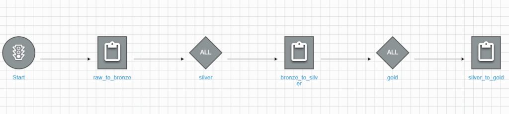
Run the created workflow and monitor the run result

1. Run the workflow.

• On the workflow detail screen –> Click Run workflow on the top.
• Wait for the response on the History tab.

2. Monitor the run result.

• On History tab –> Choose the run detail
• Choose View run details
• You can see the details of each step.

Ad-hoc queries using Athena – best way to explore the data insights

After successfully executing the glue workflow, you will see the databases and tables inside the default catalog.

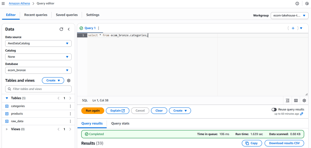
As a Data Engineer who works with SQL daily, Athena is a great tool for exploring data and executing ad-hoc queries. Let’s try on a few to test the data quality in the gold layer.

# Query I: Sales performance monitoring

WITH daily_sales AS (
    SELECT 
        d.date,
        d.day_name,
        d.is_weekend,
        SUM(f.total_sales_amount) as daily_revenue,
        SUM(f.units_sold) as daily_units,
        COUNT(DISTINCT f.product_id) as products_sold,
        AVG(f.total_sales_amount) as avg_order_value
    FROM ecom_gold.fact_sales f
    JOIN ecom_gold.dim_date d ON f.date_id = d.date_id
    GROUP BY d.date, d.day_name, d.is_weekend
)
SELECT 
    date,
    day_name,
    CASE WHEN is_weekend THEN 'Weekend' ELSE 'Weekday' END as day_type,
    daily_revenue,
    daily_units,
    products_sold,
    avg_order_value,
    -- Performance vs average
    daily_revenue / AVG(daily_revenue) OVER() as revenue_vs_avg,
    -- Running total
    SUM(daily_revenue) OVER(ORDER BY date) as cumulative_revenue
FROM daily_sales
ORDER BY date DESC;

-- Result: 
#	date	day_name	day_type	daily_revenue	daily_units	products_sold	avg_order_value	revenue_vs_avg	cumulative_revenue
1	2025-08-15	Friday	Weekday	11826422566803.00	134821851	130802	90414692.18	1.00	11826422566803.00

# Query II: Category performance & Trending

WITH category_hierarchy AS (
    SELECT 
        c.category_id,
        c.category_name,
        CASE WHEN c.parent_id IS NULL THEN c.category_name 
             ELSE parent.category_name END as parent_category,
        c.level
    FROM ecom_gold.dim_categories c
    LEFT JOIN ecom_gold.dim_categories parent ON c.parent_id = parent.category_id
),
category_performance AS (
    SELECT 
        ch.parent_category,
        ch.category_name,
        ch.level,
        COUNT(DISTINCT f.product_id) as unique_products,
        SUM(f.total_sales_amount) as category_revenue,
        SUM(f.units_sold) as category_units,
        AVG(f.total_sales_amount) as avg_sale_amount,
        -- Category metrics
        SUM(f.total_sales_amount) * 100.0 / 
            SUM(SUM(f.total_sales_amount)) OVER() as revenue_contribution_pct
    FROM ecom_gold.fact_sales f
    JOIN category_hierarchy ch ON f.category_id = ch.category_id
    GROUP BY ch.parent_category, ch.category_name, ch.level
)
SELECT 
    parent_category,
    category_name,
    level,
    unique_products,
    category_revenue,
    category_units,
    revenue_contribution_pct,
    avg_sale_amount,
    -- Performance classification
    CASE 
        WHEN revenue_contribution_pct >= 20 THEN 'Top Category'
        WHEN revenue_contribution_pct >= 10 THEN 'Major Category'
        WHEN revenue_contribution_pct >= 5 THEN 'Significant Category'
        ELSE 'Niche Category'
    END as category_importance,
    -- Efficiency metrics
    ROUND(category_revenue / unique_products, 2) as revenue_per_product,
    ROUND(category_units * 1.0 / unique_products, 2) as avg_units_per_product
FROM category_performance
ORDER BY category_revenue DESC;

# Query result:

#	parent_category	category_name	level	unique_products	category_revenue	category_units	revenue_contribution_pct	avg_sale_amount	category_importance	revenue_per_product	avg_units_per_product
1	Thời Trang Nam	Áo Khoác	1	3058	1187049355877.00	3373429	10.037264854792783	388178337.44	Major Category	388178337.44	1103.15
2	Thời Trang Nữ	Áo	1	7140	1153800931195.00	13325874	9.756128065588843	161596769.07	Significant Category	161596769.07	1866.37
3	Thời Trang Nam	Áo	1	4080	883033349352.00	6491892	7.466614222213672	216429742.49	Significant Category	216429742.49	1591.15
4	Thời Trang Nữ	Đồ lót	1	8998	824948314063.00	24818417	6.975467935490873	91681297.41	Significant Category	91681297.41	2758.21
5	Thời Trang Nữ	Quần	1	3059	627160546201.00	6797490	5.303045300964063	205021427.33	Significant Category	205021427.33	2222.13
6	Thời Trang Nam	Quần Dài/Quần Âu	1	4838	586612546195.00	3893613	4.960185913207878	121251043.03	Niche Category	121251043.03	804.8
7	Thời Trang Nữ	Áo khoác, Áo choàng & Vest	1	6060	558800593463.00	3288175	4.725017986686559	92211319.05	Niche Category	92211319.05	542.6
8	Thời Trang Nữ	Đồ tập	1	10199	544270819147.00	4475557	4.602159411035919	53365116.10	Niche Category	53365116.10	438.82
9	Thời Trang Trẻ Em	Trang phục bé gái	1	11220	439234854605.00	5356523	3.714012856583874	39147491.50	Niche Category	39147491.50	477.41
10	Thời Trang Trẻ Em	Quần áo em bé	1	10080	423106165417.00	5930642	3.5776344285605632	41974818.00	Niche Category	41974818.00	588.36
11	Thời Trang Nữ	Bộ	1	4080	359366447063.00	2444757	3.0386741640007746	88080011.54	Niche Category	88080011.54	599.21
12	Thời Trang Nam	Áo Hoodie, Áo Len & Áo Nỉ	1	3985	355766574249.00	1865083	3.008234926829384	89276430.18	Niche Category	89276430.18	468.03
13	Thời Trang Trẻ Em	Trang phục bé trai	1	10290	352913187935.00	4020415	2.9841077125523507	34296714.09	Niche Category	34296714.09	390.71
14	Thời Trang Nam	Quần Short	1	454	351132103014.00	4485185	2.969047495390827	773418729.11	Niche Category	773418729.11	9879.26
15	Thời Trang Nam	Quần Jeans	1	480	346927339969.00	2489927	2.933493522739766	722765291.60	Niche Category	722765291.60	5187.35
16	Thời Trang Nữ	Quần đùi	1	2811	323510612720.00	4113270	2.735490051134319	115087375.57	Niche Category	115087375.57	1463.28
17	Thời Trang Nữ	Đồ Bầu	1	6429	311843945945.00	3884630	2.6368408889798345	48505824.54	Niche Category	48505824.54	604.24
18	Thời Trang Nam	Đồ Lót	1	2945	287219852173.00	5924195	2.4286283578199868	97527963.39	Niche Category	97527963.39	2011.61
19	Thời Trang Nữ	Đồ ngủ	1	4080	271614181750.00	2580251	2.2966723894377523	66572103.37	Niche Category	66572103.37	632.41
20	Thời Trang Nam	Trang Phục Ngành Nghề	1	427	255008770709.00	1045791	2.1562629719050848	597210235.85	Niche Category	597210235.85	2449.16
21	Thời Trang Nữ	Hoodie và Áo nỉ	1	2277	210995255617.00	1385081	1.784100427878062	92663704.71	Niche Category	92663704.71	608.29
22	Thời Trang Nam	Đồ Bộ	1	1037	161512554017.00	1318089	1.3656923985649634	155749811.01	Niche Category	155749811.01	1271.06
23	Thời Trang Nữ	Áo len & Cardigan	1	434	159399015509.00	1772895	1.3478210727598738	367278837.58	Niche Category	367278837.58	4085.01
24	Thời Trang Nam	Áo Vest và Blazer	1	4287	157281088188.00	483377	1.3299126367215315	36687914.20	Niche Category	36687914.20	112.75
25	Thời Trang Nữ	Đồ truyền thống	1	4980	152589497378.00	784322	1.2902422225831987	30640461.32	Niche Category	30640461.32	157.49
26	Thời Trang Nữ	Vớ/ Tất	1	2994	127674136725.00	10034906	1.07956684283702	42643332.24	Niche Category	42643332.24	3351.67
27	Thời Trang Nữ	Đồ liền thân	1	4020	100583205733.00	611129	0.8504956183059028	25020697.94	Niche Category	25020697.94	152.02
28	Thời Trang Nam	Vớ/Tất	1	458	85815120230.00	5530374	0.7256219684800096	187369258.14	Niche Category	187369258.14	12075.05
29	Thời Trang Nam	Áo Ba Lỗ	1	464	81194266726.00	1498886	0.6865496837049768	174987643.81	Niche Category	174987643.81	3230.36
30	Thời Trang Nam	Trang Phục Truyền Thống	1	2751	40040590566.00	170759	0.33856891498528663	14554922.05	Niche Category	14554922.05	62.07
31	Thời Trang Nữ	Váy cưới	1	335	32651157662.00	69898	0.27608651287036234	97466142.27	Niche Category	97466142.27	208.65
32	Thời Trang Nam	Đồ Ngủ	1	445	26293147671.00	187032	0.2223254540625445	59085725.10	Niche Category	59085725.10	420.3
33	Thời Trang Nữ	Đồ hóa trang	1	426	14729052261.00	112750	0.12454359869014607	34575240.05	Niche Category	34575240.05	264.67
34	Thời Trang Nam	Đồ Hóa Trang	1	426	12216470615.00	75165	0.1032981068111998	28677161.07	Niche Category	28677161.07	176.44
35	Thời Trang Nữ	Khác	1	443	12064063588.00	134366	0.10200940749288008	27232649.18	Niche Category	27232649.18	303.31
36	Thời Trang Nam	Khác	1	312	8063453275.00	47706	0.06818167733693425	25844401.52	Niche Category	25844401.52	152.9

# Query III: Pricing strategy analysis

WITH pricing_analysis AS (
    SELECT 
        p.product_id,
        p.product_name,
        p.price,
        p.original_price,
        p.discount_rate,
        -- Discount categories
        CASE 
            WHEN p.discount_rate = 0 THEN 'No Discount'
            WHEN p.discount_rate <= 0.1 THEN 'Low Discount (≤10%)'
            WHEN p.discount_rate <= 0.2 THEN 'Medium Discount (11-20%)'
            WHEN p.discount_rate <= 0.3 THEN 'High Discount (21-30%)'
            ELSE 'Deep Discount (>30%)'
        END as discount_tier,
        -- Sales performance
        SUM(f.total_sales_amount) as total_revenue,
        SUM(f.units_sold) as total_units,
        COUNT(*) as number_of_sales
    FROM ecom_gold.dim_products p
    JOIN ecom_gold.fact_sales f ON p.product_id = f.product_id
    WHERE p.flag = true
    GROUP BY p.product_id, p.product_name, p.price, p.original_price, p.discount_rate
)
SELECT 
    discount_tier,
    COUNT(*) as products_count,
    AVG(discount_rate) as avg_discount_rate,
    SUM(total_revenue) as tier_revenue,
    SUM(total_units) as tier_units,
    AVG(total_revenue) as avg_revenue_per_product,
    AVG(total_units) as avg_units_per_product,
    -- Performance ratios
    SUM(total_revenue) * 100.0 / SUM(SUM(total_revenue)) OVER() as revenue_share_pct,
    -- Effectiveness metrics
    ROUND(SUM(total_revenue) / SUM(total_units), 2) as avg_selling_price,
    ROUND(AVG(total_revenue / NULLIF(total_units, 0)), 2) as avg_unit_revenue
FROM pricing_analysis
GROUP BY discount_tier
ORDER BY 
    CASE discount_tier
        WHEN 'No Discount' THEN 1
        WHEN 'Low Discount (≤10%)' THEN 2
        WHEN 'Medium Discount (11-20%)' THEN 3
        WHEN 'High Discount (21-30%)' THEN 4
        ELSE 5
    END;

# Query result: 
#	discount_tier	products_count	avg_discount_rate	tier_revenue	tier_units	avg_revenue_per_product	avg_units_per_product	revenue_share_pct	avg_selling_price	avg_unit_revenue
2	Low Discount (≤10%)	7074	0.06	438578844424.00	3387885	61998705.74	478.920695504665	3.7084658690879135	129455.06	237127.29
3	Medium Discount (11-20%)	10100	0.17	793677244458.00	6677683	78581905.39	661.1567326732674	6.71105095369979	118855.18	206745.12
4	High Discount (21-30%)	17319	0.27	1698597847560.00	15709886	98077131.91	907.08967030429	14.362735966563527	108122.86	170014.70
1	No Discount	34673	0.00	1516846495070.00	12133862	43747195.08	349.95131658639286	12.825911525669799	125009.37	233446.02
5	Deep Discount (>30%)	61636	0.43	7378722135291.00	96912535	119714487.24	1572.3365403335713	62.39183568497897	76137.95	140963.13

Appendix: Overview of iceberg table architecture

Because the whole series is about Lakehouse architecture based on the Iceberg table format. So, it is worth spending time to learn about the Apache Iceberg Architecture.

Let’s take dim_locations tale data in S3 as an example to discover iceberg architecture.

Find the raw dim_location files here.

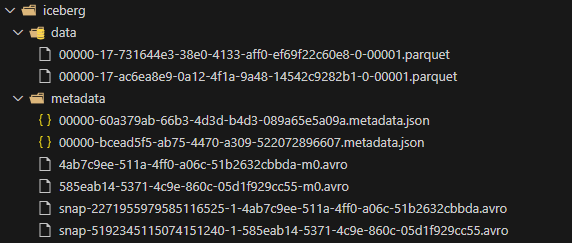
Overall Architecture

Apache Iceberg Table: dim_locations
├── data/                           # Data Layer
│   ├── 00000-17-731644e3-...-00001.parquet    # Data File 1
│   └── 00000-17-ac6ea8e9-...-00001.parquet    # Data File 2
│
└── metadata/                       # Metadata Layer
    ├── Table Metadata Files:
    │   ├── 00000-60a379ab-...metadata.json     # Table Metadata v1
    │   └── 00000-bcead5f5-...metadata.json     # Table Metadata v2 (current)
    │
    ├── Snapshot Manifests:
    │   ├── snap-2271955979585116525-1-4ab7c9ee-...avro  # Snapshot 1 Manifest
    │   └── snap-5192345115074151240-1-585eab14-...avro  # Snapshot 2 Manifest
    │
    └── Data Manifests:
        ├── 4ab7c9ee-511a-4ff0-a06c-51b2632cbbda-m0.avro # Data Manifest 1
        └── 585eab14-5371-4c9e-860c-05d1f929cc55-m0.avro # Data Manifest 2

3-Layer Metadata Architecture

1. Table Metadata (JSON)
   ├── Schema Evolution
   ├── Partition Evolution  
   ├── Snapshot History
   └── Table Properties

2. Manifest List (Avro)
   ├── Snapshot Pointers
   ├── Manifest File Lists
   └── Operation Summaries

3. Manifest Files (Avro)
   ├── Data File Inventory
   ├── File Statistics
   ├── Partition Information
   └── Column-level Metadata

Data Flow in Operations

Read Operation:

1. Read current metadata.json → Get current snapshot ID
2. Read snapshot manifest → Get list of manifest files
3. Read data manifests → Get list of data files + statistics
4. Apply predicate pushdown using statistics
5. Read relevant Parquet data files

Write Operation:

1. Write new data files to /data/
2. Create new manifest files referencing new data files
3. Create new snapshot manifest
4. Update table metadata.json with new snapshot
5. Atomic commit by updating metadata pointer

NEXT STEPS

In this article, we learned how to deploy a complete pipeline on AWS Glue based on notebooks and workflows.

In the next part, let’s learn how the Governance & Monitoring services monitor pipeline performance.