


In this blog, we’ll be looking at the calculation of functional performance metrics from the confusion matrix. The confusion matrix is specifically used for binary classifiers and we will initially concentrate on binary classification as this is the simplest starting point. With binary classification, we want our machine learning model to be able to discriminate between one of two output classes, which we typically label as positive and negative.
The following picture shows an ideal situation where the two classes are represented as similar normal distributions. Let’s imagine that our classifier will be passed images and it should discriminate between images that include cars and images that have no cars in them.
Because we are initially considering an ideal and unrealistic case, the two normal distributions do not overlap. So we can place our predicted boundary precisely between the two distributions. If we provided training and operational data like this to an algorithm, it should really be able to create a machine learning model that achieves an accuracy of 100%.

However, in the real world, life is not so easy. Machine learning systems are probabilistic and now we will see one of the reasons why this is true. In reality, we will not have two perfectly shaped normal distributions. And the contributions will also normally overlap, which creates an area of uncertainty. If a future observation occurs in this area, we cannot be sure if it is either positive or negative.
On the following section, we will use the distributions to introduce some of the terminology we use when measuring the accuracy of a binary classifier.
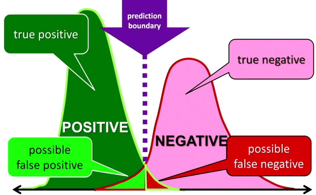
First off, let’s consider what we mean by a true positive. A true positive is where we predict that an observation is positive and it actually is positive, so we are right. This corresponds to the dark green part of the positive distribution, where any future observation will be predicted to be positive because it is to the left of the boundary and it does not overlap with the negative distribution.
Second, let’s consider the true negatives. A true negative is where we predict that an observation is negative and it is true that it is negative. So again, this means we are right. This corresponds to the pink part of the negative distribution in the above picture, where any observation will be predicted to be negative because it is to the right of the boundary and it does not overlap with the positive distribution.
When we are building models, we try to end up with models that predict as many true positives and true negatives as possible as these correspond to correctly labeled observations.
Next, we will consider false positives. A false positive is an observation where the model predicts it is positive when it is actually negative. On the picture, these can appear in the light green area of the two distributions.
Note that these ‘can’ appear rather than do appear because observations in this light green area can come from either distribution, and so some will be labeled correctly as positives and some will be incorrectly labelled as positives when they are in fact negatives. This makes them false positives. Obviously we want models that give us more true positives and fewer false positives.
Finally, we have the false negatives. These are observations labeled as negative when they are in fact positive. These can appear in the red area on the picture. Again, we are in an area of uncertainty where both distributions overlap. So some observations in this area will be labeled correctly as true negatives and some will be labeled
incorrectly as negatives when they are actually positives. These are the false negatives.
It’s worth pointing out that if you move the prediction boundary, then we change the probabilities of getting the four different results from the model. For instance, if we want zero false negatives, that is, we want the model to identify every observation that could possibly be a car as a car and never mistakenly say an image of a car was not a car.

In this case, of zero false negatives, we could move the prediction boundary to the right until there was no red area, and this would completely remove that possibility. Of course, if we did that and had zero false negatives, then the probability of false positives would correspondingly increase and our model would be far more likely to mistakenly say that an image of a bike or a horse was a car, for instance.
Confusion matrix
Here we introduce the confusion matrix, which is a table used to describe the performance of a binary classifier. The table originally comes from statistics and was subsequently used in psychology. The term confusion matrix appears to come from experiments where people did not assign items with the correct labels and so were considered to be confused.
It is not just machine learning models that get things wrong. Most humans do as well. The confusion matrix shows the four possible results from a machine learning binary classifier that we saw in the previous section.
Introduction to confusion matrix

Reading from the left, we can see that the rows correspond to the actual values. Reading from the top. We can see that the columns correspond to predicted values. In the top left of the matrix shaded in green are the True Negatives. From left of the matrix we can see that these are actually negative and from the top that they were
also predicted to be negative.
To the right, we can see that the next entry shaded in pink is a False Positive. In this row it is actually negative, but has been wrongly predicted to be positive. Below this shaded in green are the True Positives. These are actually positive and predicted to be positive.
Finally, we arrive at the False Negatives in the pink cell at the bottom left. These are actually positive but are wrongly predicted to be negative.

We want our models to generate more true predictions, which is why these are shaded in green. We also want as few as possible false predictions which are shaded in pink.
It’s worth noting that although on this confusion matrix, the actual values are shown on the left as rows and the predicted values are shown on the top as columns. It is quite possible to draw the confusion matrix with the predicted values on the rows and the actualvalues on the columns. Or we could swap the positions of the positive and negative values. It’s quite possible for confusion matrices to be drawn in different configurations and you may see different configurations from that shown on this slide in some textbooks and on web pages.
As we will see later, the configuration does not really matter as long as we are able to see which table entries are true positives, which are true negatives, which are false positives and which are false negatives.
Example of Confusion Matrix

On the above, we see an image that may well confuse our classifier, which, is trying to determine if images contain car(s) or not. This image shows an example confusion matrix for this binary image classifier. From the confusion matrix below, we can see that the classifier made 1000 predictions because the sum of all four table entries adds up to 1000. Therefore, we know that it was presented with 1000 different images to classify.
We can see that the classifier is telling us that of the 1000 observations, 880 of the images were actually not cars and only 120 were cars. It also tells us that of the 120 that were cars, 100 were correctly predicted as cars, but 20 were missed and were classified as not being a car. Of the 880 observations that were not cars, the vast majority, 850 were correctly classified as not being cars, and just 30 were wrongly classified as being a car.

In this confusion matrix, the values in the green cells far outweigh those in the pink cells, which is what we normally want. The green entries are the true positives and the true negatives, and we want the correctly predicted entries to make up the highest proportion of entries.
It’s worth to point out that although the confusion matrices we are seeing in this presentation are color coded, this is not normal practice and they are only color coded here on this blog to help in explaining how they work.
Performance metrices
We will now look at how we typically use these four values in the Matrix to generate different measures of classifier performance. Although machine learning development frameworks automatically provide us with measures of machine learning
model performance, we should also be able to calculate these metrics from the confusion matrix so that we understand what the measures are telling us.
Accuracy
On this section we introduce accuracy, which is by far the most widely used metric used for classifiers. Accuracy is very intuitive and is simply the proportion of true or green predictions.
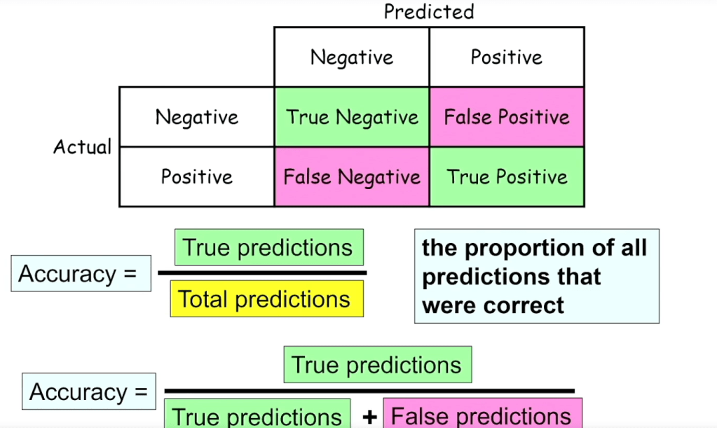
So the number of true predictions is the number of true negatives, plus the number of true positives. And the total number of predictions is the sum of all four entries in the confusion matrix.
Now we come back with the example for our car classifier. Using the car image classifier, we can see that accuracy is the proportion of true predictions. In this example, we have 950 correct predictions out of the total of 1000.And so this gives us an accuracy of 0.95 or 95%.

Precision
Precision is a separate metric that tells us how good we are at predicting positives. It measures the proportion of true positives we predict out of all positive predictions. Therefore, to achieve a higher precision, we want the number of false positives to be as low as possible. Another way to look at this is to understand that we will aim for a high precision when we do not want or cannot accept many false positives. Remember that a false positive is when we wrongly predict a positive. For instance, we predict that the image contains a car when in reality the image shows a bus.

You can imagine that in some circumstances high precision is very important. For instance, imagine we had a machine learning system that decided if you were guilty of a crime or not. Luckily, although such systems have been built and are used. So far, humans have only used them for guidance rather than allowing them to actually make decisions. As the person on trial, you would want such a system to have an extremely high or even perfect precision as you would not want it to predict you were guilty, a false positive, if there was any chance, you were not guilty.
Let’s look at an example of measuring precision for our car classifier. Using the car recognition classifier, Precision tells us how good the model is when it predicts that the image contains a car. This gives us a precision of 100 out of 130 or 0.77, which tells us that we are right 77% of the time when we predict an image as a car.

Recall (Sensitivity)
Recall or sensitivity is a separate metric that tells us how good we are at recognizing the actual positives. For a classified to do well with recall. We want the number of actual positives that are wrongly predicted to be negative, to be as low as possible. Ideally, we want all actual positives to be correctly identified.

And if we only care about recall, it does not matter how many false positives there are. So we can build a model that is very inclined to say that an observation is positive. Of course, if we do this, we may end up with a high value for recall, but we would also very likely end up with a low value for precision.
So why would we want a high value for recall?
Imagine there was a new low cost drug with no known side effects available to treat a disease that has bad consequences if not treated e.x.heart disease. If we built a machine learning model to predict who had heart disease, then we would not want there to be anyone with heart disease that was not flagged as such. That way, everyone who needed it would be prescribed the new drug.
Of course, if we build a model where we want the recall to be very high, we may find that we accidentally flag some people as potentially having the disease who do not have it. This would mean that we have a lower precision, but as the drug has no side effects and is cheap, that should not be too much of a problem.
Let’s see what the recall is for our car classifier using the car recognition classifier. Recall tells us how good we are at recognizing actual cars. This tells us that 83% of the actual cars presented to the model are recognized by the system.

Of course, this may not be acceptable if we are using the classifier to avoid hitting other cars on the road. But on the other hand, if we are using the model to automatically photograph cars as they pass us, then maybe 83% is good enough.
F1-Score (Balanced F-score, F-Measure)
The final performance metric that we will learn to calculate from the confusion matrix is the F1-score, which is also known as the balanced F-Score or F-Measure. The F one score is used when we want a balanced measure that considers both precision and recall and when there is an imbalance between the classes.

This imbalance between classes might occur. For instance, if we were trying to predict Olympic Games medal winners for a particular event and our training data was for all previous competitions. In this situation, only a small percentage of the training data examples would be labelled as medal winners and the vast majority would be labelled as losers. And so we have an imbalance between the positive and negative classes in our training data.
The F1-score provides the harmonic average of precision and recall, and the formula can be seen to be more complicated than accuracy, precision or recall, and actually uses precision and recall as part of the calculation.
Following picture is the example for the car recognition class. The highest possible F one score is one, which would mean that both recall and precision were perfect,
and the lowest possible score is zero, which would result from either of precision or recall being zero.

Conclusion
In summary, the confusion matrix is an essential tool for evaluating classification models in machine learning. By breaking down predictions into true positives, true negatives, false positives, and false negatives, it allows for the calculation of key performance metrics such as accuracy, precision, recall, F1 score, and specificity. These metrics provide deep insights into model performance, helping to identify and address errors, compare different models, and select the most appropriate one for a given task.
Understanding and utilizing these metrics is crucial for improving model accuracy and reliability in real-world applications. Whether developing spam filters or diagnostic systems, leveraging confusion matrix-derived metrics is vital for building robust and effective machine learning models.
Reference: