Efficient Data Aggregation and Grouping in Pandas

Data aggregation and grouping are crucial for data analysis, allowing us to calculate summaries and find patterns in data. Pandas makes these tasks easy and powerful with its built-in grouping and aggregation functions.

Introduction

In this blog, we’ll cover how to:

1. Use the groupby function for grouping data.
2. Perform basic aggregations like sum, mean, and count.
3. Work with multiple aggregations on multiple columns.
4. Use custom aggregation functions.
5. Leverage advanced grouping with pd.Grouper and hierarchical indexing.

We’ll be using a sample dataset to work through each of these concepts.

Setting Up Your Environment and Dataset

Start by importing Pandas and loading a sample dataset:

import pandas as pd

# Sample sales data
data = {
    'Date': pd.date_range(start='2023-01-01', periods=12, freq='ME'),
    'Store': ['Store A', 'Store B', 'Store A', 'Store B', 'Store A', 'Store B', 'Store A', 'Store B', 'Store A', 'Store B', 'Store A', 'Store B'],
    'Category': ['Electronics', 'Groceries', 'Groceries', 'Electronics', 'Groceries', 'Electronics', 'Electronics', 'Groceries', 'Groceries', 'Electronics', 'Electronics', 'Groceries'],
    'Revenue': [2300, 1500, 2000, 2600, 2100, 2300, 2800, 2400, 2700, 2200, 1900, 2100],
    'Quantity': [100, 85, 90, 120, 95, 110, 130, 115, 105, 90, 80, 100]
}

df = pd.DataFrame(data)
print("Sample Data:\n", df)

This dataset represents sales data across different stores and categories over time.

Step 1: Basic Grouping with groupby

The groupby function splits your DataFrame into groups based on some criteria. Let’s start with grouping by Store and calculating the total Revenue for each store.

# Group by 'Store' and calculate total revenue
store_revenue = df.groupby('Store')['Revenue'].sum()
print("Total Revenue by Store:\n", store_revenue)

This outputs the total revenue for each store, giving us an overview of sales per store.

Step 2: Grouping by Multiple Columns

You can group by multiple columns to get more granular insights. Let’s calculate total Revenue by Store and Category.

# Group by 'Store' and 'Category' and calculate total revenue
store_category_revenue = df.groupby(['Store', 'Category'])['Revenue'].sum()
print("Total Revenue by Store and Category:\n", store_category_revenue)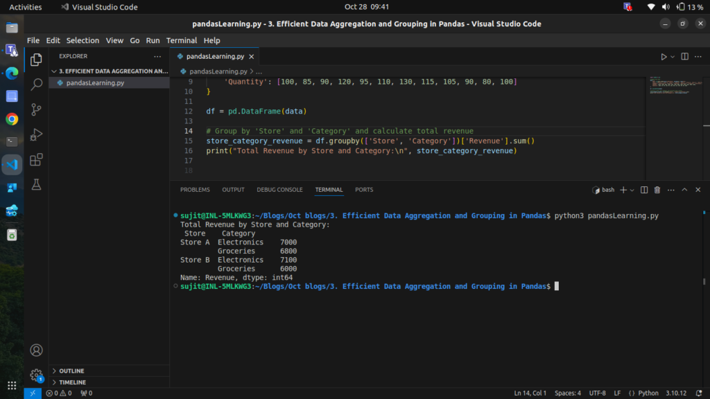

This gives the revenue split not only by store but also by category, letting us see which categories perform well at each store.

Step 3: Using Aggregate Functions on Multiple Columns

We can perform multiple aggregations on different columns simultaneously. Let’s find both the total and average Revenue and Quantity for each store.

# Group by 'Store' and aggregate 'Revenue' and 'Quantity' with sum and mean
store_aggregates = df.groupby('Store').agg({
    'Revenue': ['sum', 'mean'],
    'Quantity': ['sum', 'mean']
})
print("Aggregated Revenue and Quantity by Store:\n", store_aggregates)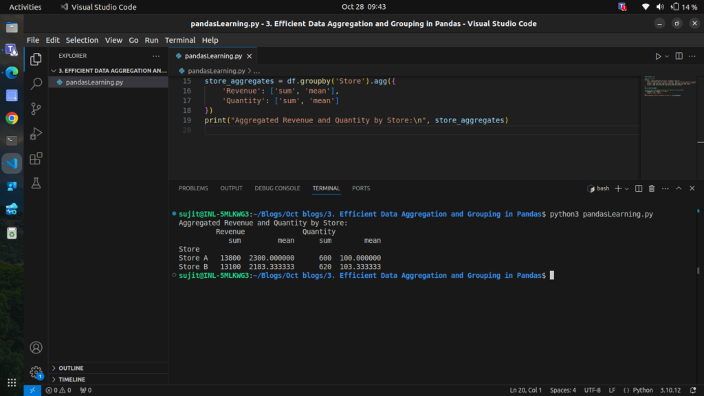

Here, we get the total and average revenue and quantity per store, providing a more detailed picture of performance.

Step 4: Custom Aggregation Functions

You can apply custom functions within agg to perform specialized calculations. Let’s use a custom function to calculate the range (max – min) for Revenue

# Define a custom function to calculate range
def calculate_range(x):
    return x.max() - x.min()

# Group by 'Store' and apply custom aggregation for revenue range
store_revenue_range = df.groupby('Store').agg({'Revenue': calculate_range})
print("Revenue Range by Store:\n", store_revenue_range)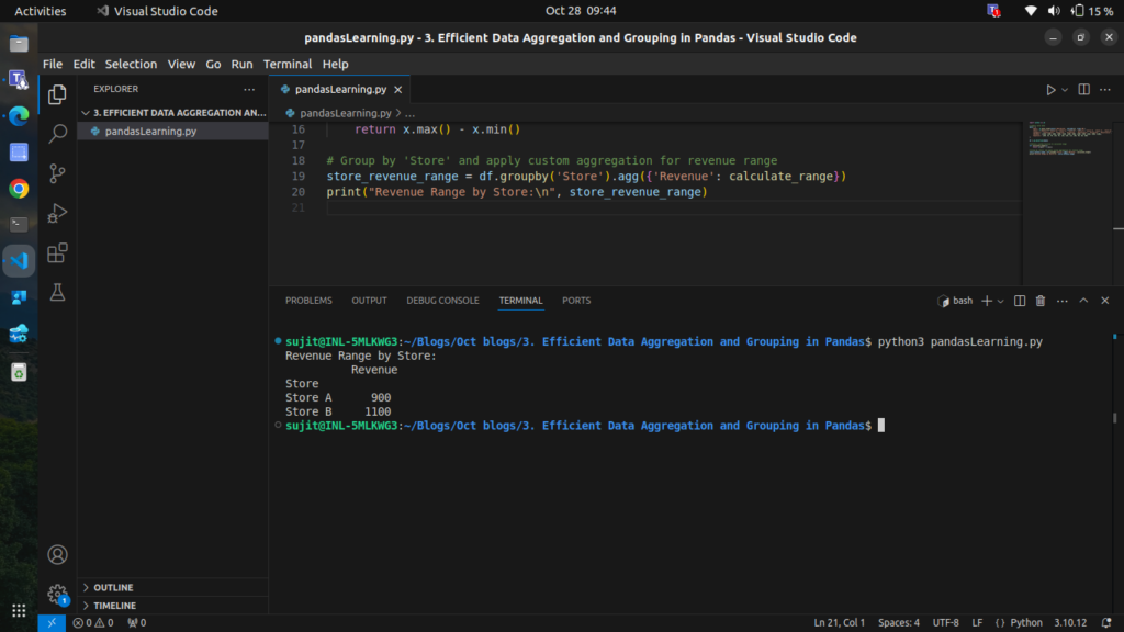

This custom aggregation allows us to see the fluctuation in revenue for each store

Step 5: Grouping by Date with pd.Grouper

pd.Grouper helps group by time-based data. For instance, let’s calculate monthly total Revenue across all stores.

# Set 'Date' as the index to enable time-based grouping
df.set_index('Date', inplace=True)

# Group by month and calculate total revenue
monthly_revenue = df.groupby(pd.Grouper(freq='ME'))['Revenue'].sum()
print("Monthly Total Revenue:\n", monthly_revenue)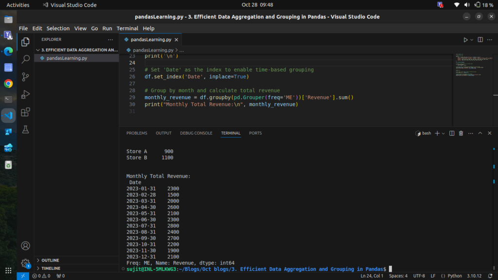

This aggregates the data on a monthly basis, providing insight into revenue trends over time.

Step 6: Grouping with Hierarchical Indexing

When grouping by multiple columns, Pandas returns a DataFrame with a multi-level index, also known as a hierarchical index. Let’s explore how to handle this by grouping Store and Category, then performing aggregation.

# Group by 'Store' and 'Category' and calculate total and average revenue
hierarchical_group = df.groupby(['Store', 'Category']).agg({
    'Revenue': ['sum', 'mean'],
    'Quantity': 'sum'
})
print("Hierarchical Grouping by Store and Category:\n", hierarchical_group)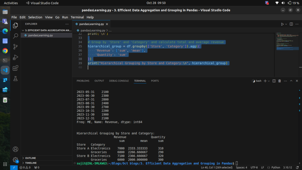

The result is a DataFrame with a multi-level index (Store and Category), allowing us to drill down into specific group details.

Step 7: Transforming Grouped Data

transform allows you to apply a function to each group independently and return a result that aligns with the original DataFrame. For instance, let’s normalize Revenue within each store.

# Group by 'Store' and normalize 'Revenue' within each store
df['Normalized_Revenue'] = df.groupby('Store')['Revenue'].transform(lambda x: (x - x.mean()) / x.std())
print("DataFrame with Normalized Revenue by Store:\n", df)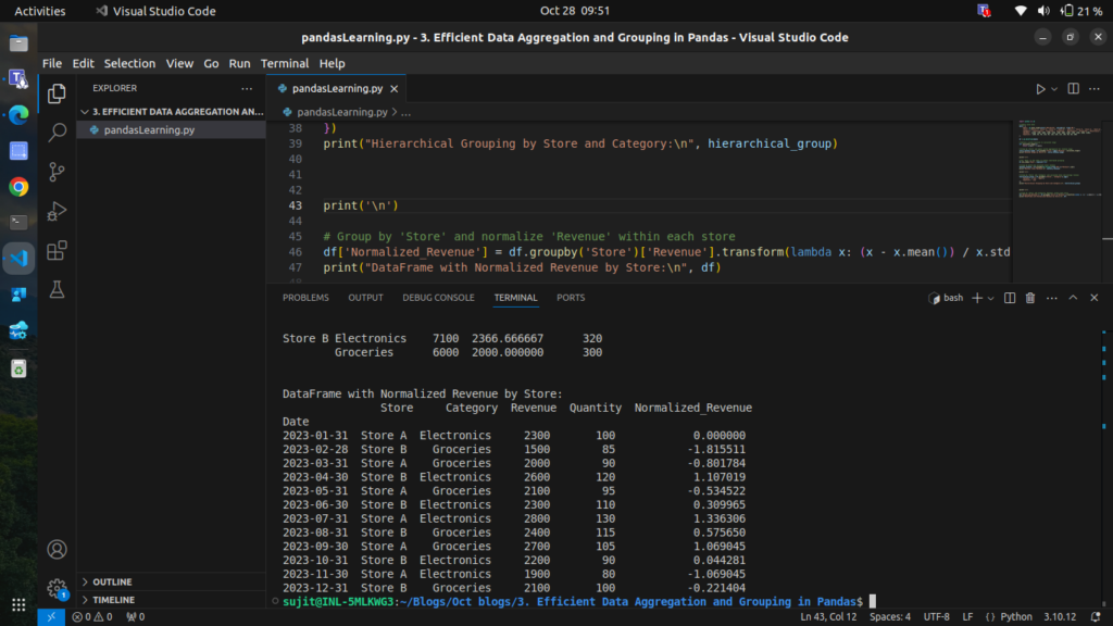

This gives each store’s revenue a relative scale, making it easier to compare performance within each store.

Step 8: Filtering Groups with filter

Sometimes, you may want to filter groups based on a condition. For example, let’s keep only those stores with an average Revenue above 2000.

# Filter groups to keep only stores with average revenue > 2000
filtered_df = df.groupby('Store').filter(lambda x: x['Revenue'].mean() > 2000)
print("Filtered DataFrame (Stores with Avg Revenue > 2000):\n", filtered_df)

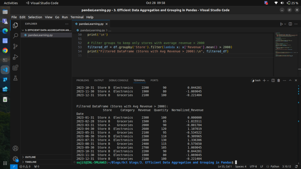
This filters out any groups where the condition isn’t met, leaving only the data we want.

you can access complete code of this blog from here:

import pandas as pd

# Sample sales data
data = {
    'Date': pd.date_range(start='2023-01-01', periods=12, freq='ME'),
    'Store': ['Store A', 'Store B', 'Store A', 'Store B', 'Store A', 'Store B', 'Store A', 'Store B', 'Store A', 'Store B', 'Store A', 'Store B'],
    'Category': ['Electronics', 'Groceries', 'Groceries', 'Electronics', 'Groceries', 'Electronics', 'Electronics', 'Groceries', 'Groceries', 'Electronics', 'Electronics', 'Groceries'],
    'Revenue': [2300, 1500, 2000, 2600, 2100, 2300, 2800, 2400, 2700, 2200, 1900, 2100],
    'Quantity': [100, 85, 90, 120, 95, 110, 130, 115, 105, 90, 80, 100]
}

# Create DataFrame
df = pd.DataFrame(data)
print("Sample Data:\n", df)

# Step 1: Basic Grouping with `groupby`
store_revenue = df.groupby('Store')['Revenue'].sum()
print("\nTotal Revenue by Store:\n", store_revenue)

# Step 2: Grouping by Multiple Columns
store_category_revenue = df.groupby(['Store', 'Category'])['Revenue'].sum()
print("\nTotal Revenue by Store and Category:\n", store_category_revenue)

# Step 3: Using Aggregate Functions on Multiple Columns
store_aggregates = df.groupby('Store').agg({
    'Revenue': ['sum', 'mean'],
    'Quantity': ['sum', 'mean']
})
print("\nAggregated Revenue and Quantity by Store:\n", store_aggregates)

# Step 4: Custom Aggregation Functions
def calculate_range(x):
    return x.max() - x.min()

store_revenue_range = df.groupby('Store').agg({'Revenue': calculate_range})
print("\nRevenue Range by Store:\n", store_revenue_range)

# Step 5: Grouping by Date with `pd.Grouper`
df.set_index('Date', inplace=True)
monthly_revenue = df.groupby(pd.Grouper(freq='ME'))['Revenue'].sum()
print("\nMonthly Total Revenue:\n", monthly_revenue)

# Step 6: Grouping with Hierarchical Indexing
hierarchical_group = df.groupby(['Store', 'Category']).agg({
    'Revenue': ['sum', 'mean'],
    'Quantity': 'sum'
})
print("\nHierarchical Grouping by Store and Category:\n", hierarchical_group)

# Step 7: Transforming Grouped Data
df['Normalized_Revenue'] = df.groupby('Store')['Revenue'].transform(lambda x: (x - x.mean()) / x.std())
print("\nDataFrame with Normalized Revenue by Store:\n", df)

# Step 8: Filtering Groups with `filter`
filtered_df = df.groupby('Store').filter(lambda x: x['Revenue'].mean() > 2000)
print("\nFiltered DataFrame (Stores with Avg Revenue > 2000):\n", filtered_df)

Conclusion

This blog covers efficient data aggregation and grouping techniques in Pandas, from basic grouping to advanced methods like custom aggregations, hierarchical indexing, and time-based grouping. Mastering these techniques will enable you to analyze large datasets efficiently and extract valuable insights.