


In the realm of machine learning, Generative Adversarial Networks (GANs) have emerged as a groundbreaking technique that revolutionises the way we generate and understand data. GANs enable us to generate realistic synthetic samples by pitting two neural networks against each other, resulting in astonishingly impressive outputs. In this blog post, we will dive deep into the world of GANs, unravelling their inner workings, applications, and future potential.
Understanding What are GANs
Generative Adversarial Networks (GANs)offer a unique approach to generate new datasets by learning from existing training data. Comprising two neural networks, namely generators and discriminators. GANs engage in a competitive game to capture, replicate, and analyze the variations present within a dataset. GAN Components: Generative, Controversial, and Networks:
Generative: GANs excel at learning generative models that depict how data is probabilistically generated. These models provide visual explanations of the data generation process, enabling a deeper understanding of its underlying patterns.
Adversarial: GANs are trained in a hostile environment where the generator network competes against the discriminator network. This adversarial training fosters continuous improvement in both networks resulting in enhanced performance and realistic sample generation.
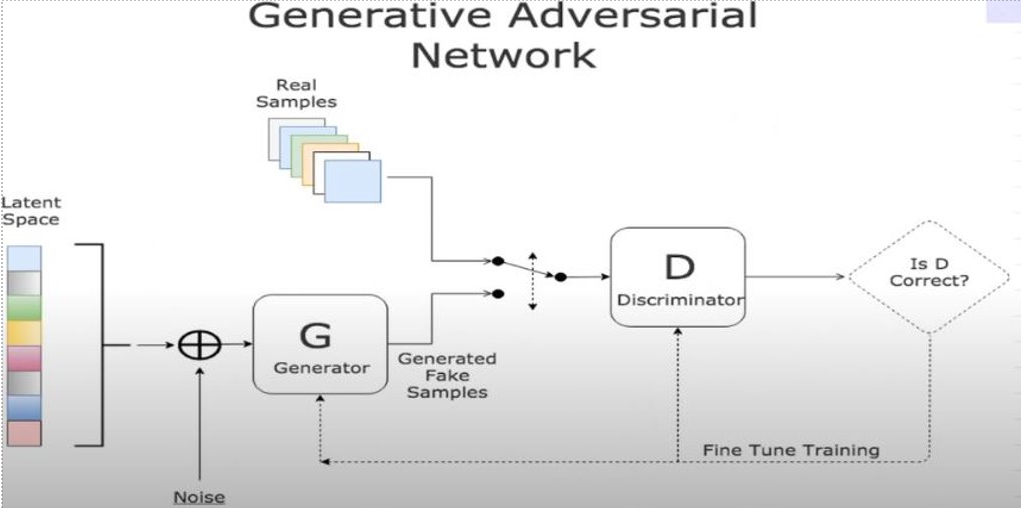
Networks: GANs leverage the power of deep neural networks for training purposes. The generator network takes random input, often noise and generates samples such as images, text, or audio that closely resemble the training data. On the other hand, the discriminator network aims to differentiate between real and generated samples. Effectively classifying genuine data as real and generated data as fake.
Why GANS
Machine learning algorithms and neural networks can be prone to misclassifications when exposed to noisy data. Adding noise to the data increases the likelihood of misclassification. To address this issue, researchers have explored techniques to enhance neural networks’ visualization capabilities, allowing them to recognize new patterns similar to the training data. One such technique involves using Generative Adversarial Networks (GANs), which generate synthetic results that closely resemble the original data.
GANs Components
In a Generative Adversarial Network (GAN), there are two key components: the generator and the discriminator. These components work in tandem to create a competitive learning framework that leads to the generation of realistic synthetic data.
Generator
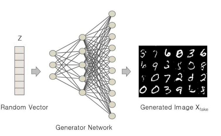
The generator is a crucial component of a Generative Adversarial Network (GAN). Its primary role is to generate synthetic samples that resemble real data. By taking random noise as input, the generator aims to transform it into meaningful and realistic data that closely matches the distribution of the training data.
The generator operates by learning a mapping from a latent space to the data space. The latent space is a lower-dimensional representation that captures the underlying patterns and features of the data. The generator’s objective is to capture these patterns and generate outputs that are indistinguishable from real data samples.
To achieve this, the generator is typically designed as a neural network. It takes the random noise vector, often drawn from a probability distribution such as a uniform or Gaussian distribution, as its input. This noise vector serves as a source of randomness and variability, allowing the generator to produce diverse outputs.
The neural network architecture of the generator consists of layers of interconnected nodes, also known as neurons. Each neuron performs a mathematical transformation on its input, which is passed through an activation function to introduce non-linearity. The activation functions help the generator capture complex relationships and generate diverse data.
During training, the generator improves its ability to generate synthetic data that closely resembles real samples. It captures intricate details, patterns, and variations from the training set, aiming for generated samples that are virtually indistinguishable from real ones. Factors such as network architecture, activation functions, dataset size, complexity, and optimization techniques impact the generator’s ability to produce high-quality synthetic data.
Discriminator
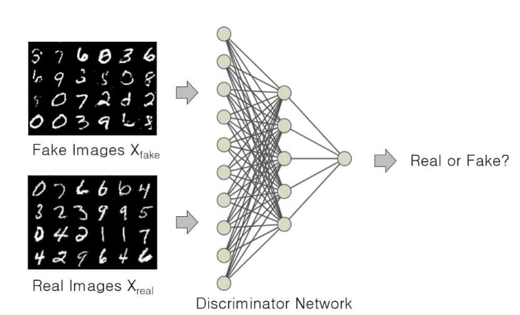
The discriminator is a vital component of a Generative Adversarial Network (GAN) responsible for distinguishing real and generated data samples. It acts as a binary classifier, learning to differentiate between the two types of samples based on their distinct characteristics.
Implemented as a neural network, the discriminator receives both real data from the training set and generated samples from the generator. Through training, it refines its ability to accurately classify the samples by updating its parameters.
During the training process, the discriminator compares the generated samples to the real ones and provides feedback to the generator. This feedback helps the generator improve its output quality over time.
By adjusting its parameters using techniques like backpropagation. The discriminator learns to identify subtle patterns and differences that distinguish real data from generated data. Its goal is to become a formidable adversary for the generator. Making it challenging to produce samples that fool the discriminator.
Factors such as network architecture, choice of activation functions, dataset size, complexity, and optimization techniques influence the discriminator’s performance. As training progresses, the discriminator’s discriminatory abilities improve, aiding in the competition and guiding the overall learning process of the GAN.
In summary, the discriminator’s role is to differentiate between real and generated samples. Providing feedback to the generator and driving the GAN towards generating high-quality synthetic data that closely resembles real data.
Training Procedure
To understand the training process of a GAN, we will delve into the detailed steps involved. Firstly, it is crucial to define the specific problem the GAN aims to solve, such as generating audio, poems, text, or images. Secondly, selecting an appropriate GAN architecture becomes important, given the various types available.
The training begins with the discriminator, which is exposed solely to real images, enabling it to accurately classify them. Forward propagation is employed, without backpropagation, and the discriminator’s weights are updated based on its performance. Penalizing the misclassification of real and fake data through the discriminator loss enhances its ability to differentiate between the two.
Next, the generator undergoes training by taking random noise as input and transforming it into meaningful data, generating fake outputs. Meanwhile, the discriminator remains idle. Training the generator involves predicting its output from the discriminator’s perspective, calculating the discriminator loss. Gradients are computed through backpropagation on both the discriminator and generator, facilitating the update of the generator’s weights.
Subsequently, the discriminator is trained on the fake data produced by the generator. It assesses whether the data is fake or real and provides feedback to the generator, forming a feedback loop that enhances the generator’s output quality.
The training process for both the generator and discriminator continues iteratively, with each component taking turns being trained. This iterative process fosters the refinement of the generator’s ability to generate more realistic outputs and the discriminator’s ability to accurately classify real and fake data.
In summary, GAN training involves initially training the discriminator on real data, followed by training the generator to improve its output quality with the generation of fake data. Subsequently, the discriminator is trained on the generated data, providing feedback to the generator.
Loss Function
A loss function is a mathematical function that measures the difference between the predicted output of a machine learning model and the actual output.In GANs, there are two loss functions: the generator loss and the discriminator loss
Generator loss
- The generator loss measures how well the generator is able to create realistic-looking fake data that can fool the discriminator.
- Typically, one calculates the generator loss by computing the difference between the generated data and the real data.
- The generator loss updates the generator weights to enhance the quality of the generated data.
- Generator Loss Formula: Lᴳ = -𝔼[log(D(G(z)))]
Discriminator loss
- The discriminator loss measures how well the discriminator is able to distinguish between real and fake data.
- The discriminator loss updates the discriminator weights to enhance its ability to differentiate between real and fake data.
- It penalizes itself for misclassifying a real instance as fake, or a fake instance (created by the generator) as real, by maximizing the below function.
- Discriminator Loss Formula: Lᴰ = -𝔼[log(D(x))] – 𝔼[log(1 – D(G(z)))]
Implementation Of GANS using Tensorflow
import os
import time
import numpy as np
import tensorflow as tf
from tensorflow.keras import layers
from IPython import display
import matplotlib.pyplot as plt
# %matplotlib inline
from tensorflow import keras
x_train.shape
BUFFER_SIZE = 60000
BATCH_SIZE = 128
latent_dim = 100
image_dim = 784
num_examples_to_generate = 25
# We will reuse this seed overtime to visualize progress
seed = tf.random.normal([num_examples_to_generate, latent_dim])
def generator(image_dim):
inputs = keras.Input(shape=(100,), name='input_layer')
x = layers.Dense(128, kernel_initializer=tf.keras.initializers.he_uniform, name='dense_1')(inputs)
#print(x.dtype)
x = layers.LeakyReLU(0.2, name='leaky_relu_1')(x)
x = layers.Dense(256, kernel_initializer=tf.keras.initializers.he_uniform, name='dense_2')(x)
x = layers.BatchNormalization(momentum=0.1, epsilon=0.8, name='bn_1')(x)
x = layers.LeakyReLU(0.2, name='leaky_relu_2')(x)
x = layers.Dense(512, kernel_initializer=tf.keras.initializers.he_uniform, name='dense_3')(x)
x = layers.BatchNormalization(momentum=0.1, epsilon=0.8, name='bn_2')(x)
x = layers.LeakyReLU(0.2, name='leaky_relu_3')(x)
x = layers.Dense(1024, kernel_initializer=tf.keras.initializers.he_uniform, name='dense_4')(x)
x = layers.BatchNormalization(momentum=0.1, epsilon=0.8, name='bn_3')(x)
x = layers.LeakyReLU(0.2, name='leaky_relu_4')(x)
x = layers.Dense(image_dim, kernel_initializer=tf.keras.initializers.he_uniform, activation='tanh', name='dense_5')(x)
outputs = tf.reshape(x, [-1, 28, 28, 1], name='Reshape_Layer')
model = tf.keras.Model(inputs, outputs, name="Generator")
return model
generator = generator(image_dim)
generator.summary()
def discriminator():
inputs = keras.Input(shape=(28,28,1), name='input_layer')
input = tf.reshape(inputs, [-1, 784], name='reshape_layer')
x = layers.Dense(512, kernel_initializer=tf.keras.initializers.he_uniform, name='dense_1')(input)
x = layers.LeakyReLU(0.2, name='leaky_relu_1')(x)
x = layers.Dense(256, kernel_initializer=tf.keras.initializers.he_uniform, name='dense_2')(x)
x = layers.LeakyReLU(0.2, name='leaky_relu_2')(x)
outputs = layers.Dense(1, kernel_initializer=tf.keras.initializers.he_uniform, activation='sigmoid', name='dense_3') (x)
model = tf.keras.Model(inputs, outputs, name="Discriminator")
return model
discriminator = discriminator()
discriminator.summary()
#Loss function
binary_cross_entropy = tf.keras.losses.BinaryCrossentropy()
def generator_loss(fake_output):
gen_loss = binary_cross_entropy(tf.ones_like(fake_output), fake_output)
#print(gen_loss)
return gen_loss
def discriminator_loss(real_output, fake_output):
real_loss = binary_cross_entropy(tf.ones_like(real_output), real_output)
fake_loss = binary_cross_entropy(tf.zeros_like(fake_output), fake_output)
total_loss = real_loss + fake_loss
#print(total_loss)
return total_loss
learning_rate = 0.0002
generator_optimizer = tf.keras.optimizers.Adam(learning_rate = 0.0002, beta_1 = 0.5, beta_2 = 0.999 )
discriminator_optimizer = tf.keras.optimizers.Adam(learning_rate = 0.0002, beta_1 = 0.5, beta_2 = 0.999 )
# Notice the use of `tf.function`
# This annotation causes the function to be "compiled".
@tf.function
def train_step(images):
noise = tf.random.normal([BATCH_SIZE, latent_dim])
with tf.GradientTape() as gen_tape, tf.GradientTape() as disc_tape:
generated_images = generator(noise, training=True)
real_output = discriminator(images, training=True)
fake_output = discriminator(generated_images, training=True)
gen_loss = generator_loss(fake_output)
disc_loss = discriminator_loss(real_output, fake_output)
gradients_of_gen = gen_tape.gradient(gen_loss, generator.trainable_variables)
gradients_of_disc = disc_tape.gradient(disc_loss, discriminator.trainable_variables)
generator_optimizer.apply_gradients(zip(gradients_of_gen,\
generator.trainable_variables))
discriminator_optimizer.apply_gradients(zip(gradients_of_disc,\
discriminator.trainable_variables))
#return gen_loss, disc_loss
!mkdir tensor
import os
checkpoint_dir = './training_checkpoints'
checkpoint_prefix = os.path.join(checkpoint_dir, "ckpt")
checkpoint = tf.train.Checkpoint(generator_optimizer=generator_optimizer,
discriminator_optimizer=discriminator_optimizer,
generator=generator,
discriminator=discriminator)
def train(dataset, epochs):
for epoch in range(epochs):
start = time.time()
i = 0
D_loss_list, G_loss_list = [], []
for image_batch in dataset:
i += 1
train_step(image_batch)
display.clear_output(wait=True)
generate_and_save_images(generator,
epoch + 1,
seed)
# Save the model every 15 epochs
if (epoch + 1) % 15 == 0:
checkpoint.save(file_prefix = checkpoint_prefix)
print ('Time for epoch {} is {} sec'.format(epoch + 1, time.time()-start))
# Generate after the final epoch
display.clear_output(wait=True)
generate_and_save_images(generator,
epochs,
seed)
def generate_and_save_images(model, epoch, test_input):
# Notice `training` is set to False.
# This is so all layers run in inference mode (batchnorm).
predictions = model(test_input, training=False)
#print(predictions.shape)
fig = plt.figure(figsize=(4,4))
for i in range(predictions.shape[0]):
plt.subplot(5, 5, i+1)
pred = (predictions[i, :, :, 0] + 1) * 127.5
pred = np.array(pred)
plt.imshow(pred.astype(np.uint8), cmap='gray')
plt.axis('off')
plt.savefig('tensor/image_at_epoch_{:d}.png'.format(epoch))
plt.show()
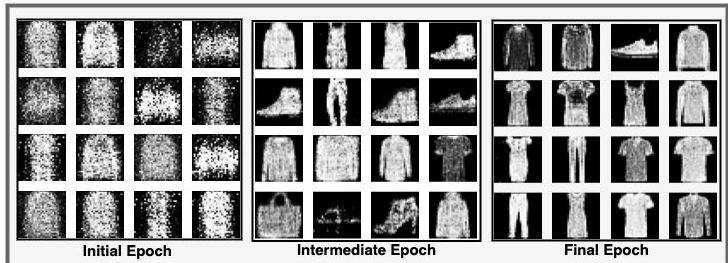
#Generate images
train(train_dataset, 50)Results
Link to Dataset : https://www.tensorflow.org/datasets/catalog/mnist
Conclusion
Generative Adversarial Networks offer a powerful approach to generative modeling by employing a unique interplay between two neural networks: the generator and discriminator. Through adversarial training, GANs enable the generation of realistic samples that closely resemble the training data. By understanding the components and training process of GANs, we can appreciate the profound impact they have had on various fields, including computer vision, natural language processing, and audio synthesis.